

Sub1Hour
Veteran
I'm not quite sure how many people on these forums can appreciate this, but for the few of you, I think you will enjoy this analysis for what it is. Basically, I wanted to compare an average of 25 in 3x3 and square-1 to find out which one I'm actually faster in. I'll post it as a spoiler since its a couple of pages.
It's still a little rough around the edges but I think I used enough material from my AP Stats course within it to get a good mark.
You may not know this, but I am an avid fanatic of twisty puzzles. You may know the “original” and most famous twisty puzzle, Rubik’s Cube. There are competitions worldwide where people like me try and solve their puzzles as quickly as possible. I have been solving puzzles like these for over 5 years and I am currently a trainee delegate for the WCA, the governing body of these competitions. My personal favorite event is Square-1, an atypical puzzle characterized by its shape-shifting capabilities. I currently average around 11 seconds on this puzzle, but I also average around 11 seconds on the classic 3x3 Rubik’s cube. I will be timing 25 solves of each puzzle and comparing the data. I will give myself 10 warm-up solves for each puzzle that will not go into the final statistical analysis. All of these solves will be done in a controlled environment at room temperature and minimal noise to ensure equal conditions for both sets of data. All scrambles for these puzzles will be generated using the latest version of CSTimer, utilizing random-state scrambles. I will be using a Speedstacks gen 5 timer, which is the latest version of the Speedstacks timer and is the most widely used in WCA competitions.
My Hypothesis is that I will be slightly faster on Square-1, but have a much larger standard deviation due to parity, a phenomenon on square-1 that allows for only 2 pieces to be swapped, which requires a long algorithm to fix that can add seconds to an otherwise fast time. This occurs on average every 1 in 2 solves for me, as I do not currently know the method to avoid odd parity cases. This will cause the standard deviation and the spread to be much larger for my square-1 data set compared to my 3x3 set. The Null Hypothesis I will be setting is as follows, with s representing my Square-1 data and r representing my 3x3 or “Rubik’s Cube” Data
H0 μs = μr
My alternative hypothesis is as follows.
Ha μs < μr
Keep in mind that a faster time is viewed as better, so a smaller mean would equate to a better time.
Now, It’s time to bring in the results. I will begin by doing my 3x3 solves, then my Square-1 Solves
Here is the data that was produced.
The software (CSTimer) that I used has a very useful statistics tool that can provide us with a few values that will display the general variance and mean of each data set.
Here is the data for the 3x3 set
μ = 12.04, σ = 1.44, min = 9.00, max = 18.84, Q1 = 10.52 , Median = 11.23, Q3 = 12.70
Here is the data for the Square-1 Set
μ = 11.63, σ = 1.49, min = 8.79, max = 15.58, Q1 = 10.41, Median = 11.30, Q3 = 13.19
And here is a box plot depicting both data sets
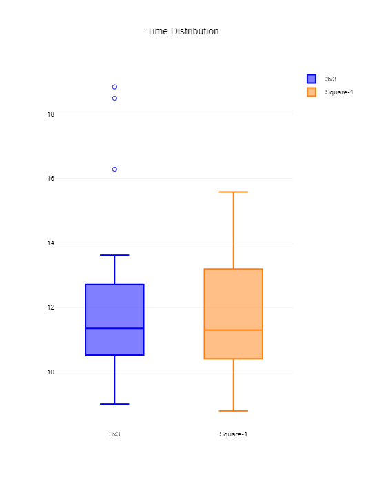
Based on the data and my assumptions prior to testing, I am not surprised by the box plots. The slightly larger IQR on the square-1 plot was predicted, however, the median is slightly slower in square-1 despite the mean being slightly faster than 3x3. I am however surprised that there were outliers found in the 3x3 data and not the square-1 data. I was expecting to have at least 1 outlier in square-1 due to the nature of parity and “bad” solves being more common in this event compared to 3x3. The presence of outliers in the 3x3 data was not expected but it does indicate that the “bad” solve in 3x3 are much worse than the bad solves in the square-1 data in this data set.
I will now use a statistical test to figure out if the null hypothesis is true or not. The test I will be using is a 2 sample T-test.
By performing this test with the condition of μ1 =/= μ2, with μ1 being the 3x3 data and μ2 being the square-1 data, we get the p value of .3274, causing us to fail to reject the null hypothesis at an alpha level of 0.05. The values are simply too close together for a clear answer to be given by using a 2 sample T test, however, there is still a difference between both data sets that suggests that the null hypothesis is false. By running this test with a condition of μ1 > μ2 we can receive the P value of .1637, which means that we also fail to reject the alternative hypothesis, assuming that the alternative hypothesis takes the place of the null hypothesis when conducting the 2 sample T-test.
Overall I am very happy with the results of this analysis. I’ve loved to see my improvement progress at nearly identical rates for both events for a while now, and this only shows me that the times are even closer than I would’ve imagined.
My Hypothesis is that I will be slightly faster on Square-1, but have a much larger standard deviation due to parity, a phenomenon on square-1 that allows for only 2 pieces to be swapped, which requires a long algorithm to fix that can add seconds to an otherwise fast time. This occurs on average every 1 in 2 solves for me, as I do not currently know the method to avoid odd parity cases. This will cause the standard deviation and the spread to be much larger for my square-1 data set compared to my 3x3 set. The Null Hypothesis I will be setting is as follows, with s representing my Square-1 data and r representing my 3x3 or “Rubik’s Cube” Data
H0 μs = μr
My alternative hypothesis is as follows.
Ha μs < μr
Keep in mind that a faster time is viewed as better, so a smaller mean would equate to a better time.
Now, It’s time to bring in the results. I will begin by doing my 3x3 solves, then my Square-1 Solves
Here is the data that was produced.
| 3x3 Times | Square-1 Times |
| 10.11 | 11.57 |
| 11.48 | 10.42 |
| 10.57 | 10.65 |
| 10.40 | 13.31 |
| 12.68 | 10.47 |
| 10.77 | 12.88 |
| 9.00 | 13.18 |
| 12.79 | 8.79 |
| 18.84 | 10.16 |
| 11.07 | 11.30 |
| 11.62 | 14.30 |
| 18.49 | 14.34 |
| 12.11 | 11.13 |
| 11.49 | 11.06 |
| 16.285 | 13.22 |
| 13.62 | 13.67 |
| 11.15 | 10.37 |
| 11.35 | 10.60 |
| 13.08 | 9.20 |
| 10.40 | 12.18 |
| 12.23 | 15.58 |
| 9.36 | 13.03 |
| 10.33 | 8.98 |
| 10.56 | 11.34 |
| 11.31 | 9.12 |
The software (CSTimer) that I used has a very useful statistics tool that can provide us with a few values that will display the general variance and mean of each data set.
Here is the data for the 3x3 set
μ = 12.04, σ = 1.44, min = 9.00, max = 18.84, Q1 = 10.52 , Median = 11.23, Q3 = 12.70
Here is the data for the Square-1 Set
μ = 11.63, σ = 1.49, min = 8.79, max = 15.58, Q1 = 10.41, Median = 11.30, Q3 = 13.19
And here is a box plot depicting both data sets
Based on the data and my assumptions prior to testing, I am not surprised by the box plots. The slightly larger IQR on the square-1 plot was predicted, however, the median is slightly slower in square-1 despite the mean being slightly faster than 3x3. I am however surprised that there were outliers found in the 3x3 data and not the square-1 data. I was expecting to have at least 1 outlier in square-1 due to the nature of parity and “bad” solves being more common in this event compared to 3x3. The presence of outliers in the 3x3 data was not expected but it does indicate that the “bad” solve in 3x3 are much worse than the bad solves in the square-1 data in this data set.
I will now use a statistical test to figure out if the null hypothesis is true or not. The test I will be using is a 2 sample T-test.
By performing this test with the condition of μ1 =/= μ2, with μ1 being the 3x3 data and μ2 being the square-1 data, we get the p value of .3274, causing us to fail to reject the null hypothesis at an alpha level of 0.05. The values are simply too close together for a clear answer to be given by using a 2 sample T test, however, there is still a difference between both data sets that suggests that the null hypothesis is false. By running this test with a condition of μ1 > μ2 we can receive the P value of .1637, which means that we also fail to reject the alternative hypothesis, assuming that the alternative hypothesis takes the place of the null hypothesis when conducting the 2 sample T-test.
Overall I am very happy with the results of this analysis. I’ve loved to see my improvement progress at nearly identical rates for both events for a while now, and this only shows me that the times are even closer than I would’ve imagined.
It's still a little rough around the edges but I think I used enough material from my AP Stats course within it to get a good mark.


